The paper published by J. de la Porte¹, B. M. Herbst¹, W. Hereman² and S. J. van der Walt¹ in November 2008 describes the mathematical technique for dealing with reducing dimensionality in data. In that paper, the authors give an overview of three well-known dimensionality reduction techniques and introduce diffusion maps and its functionality, process and how it compares with the other methods.

Dimensionality Reduction

We are limited in visualising information beyond the third dimension. For simplicity reasons, imagine a black and white image (grey scale) of 100 by 100 pixels, where each pixel represents a variable. The dimensionality would add up to be 10,000. A human would not have any issues with reading the following digits in the picture below, but a computer sees them as a data point in an nm-dimensional coordinate space.

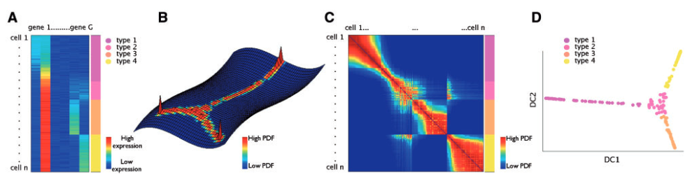
Dimensionality reduction is about converting data of very high dimensionality into data of lower dimensionality while preserving the original information. We can achieve these if one would be able to measure the distance between data points on the manifold itself instead of in Euclidean space by taking into account the data global space.

We can use the analogy of zipping text files, compressing large text data into smaller equivalent data. With the minor but significant difference that in dimensionality reduction we will lose some information. The goal here is to not lose too many of the essential features in the data.

Popular Techniques

The most popular reduction methods are

• Principle Component Analysis (PCA)³, a linear dimensionality reduction technique using Singular Value Decomposition of the data to project it to a lower dimensional space.⁴
• Multi-dimensional Scaling (MDS)⁵ seeks a low-dimensional representation of the data in which the distances respect well the distances in the original high-dimensional space.⁶
• Isometric Feature Map (Isomap)⁷, a non-linear dimensionality reduction through Isometric Mapping.⁸

Diffusion Maps

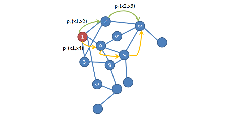
Diffusion maps are a non-linear technique. Similar to taking a random walk on our data, where we jump between data points in feature space (see image below), we are analysing the connectivity of the data. The goal is to reveal the geometric structure of our data at different scales, defining a “time-dependent” diffusion metrics.

By measuring the distances between data points (i.e. Euclidean space), we can define neighbourhoods. In order to achieve it, we define a threshold value in the way of a function (kernel) to obtain the similarity within the geometric structure, which allows us to preserve the underlying information of the given data and be able to connect each neighbourhood.

The basic diffusion mapping algorithm can be defined as follows:

INPUT: High dimensional data set

1. Define a kernel, \(k(x, y)\) and create a kernel matrix, $K$, such that \(K_{i,j} = k(X_i, X_j)\).
2. Create the diffusion matrix by normalising the rows of the kernel matrix
3. Calculate the eigenvectors of the diffusion matrix.
4. Map to the \(d\)-dimensional diffusion space at time \(t\), using the \(d\) dominant eigenvectors and -values

OUTPUT: Lower dimensional data set

Comparison

The authors also investigated the performance of the different algorithms using a data set with an underlying C-shape for the change of the parameters. As for PCA, once the data is projected onto the two primary axes of variation the ordering of the data along the non-linear C-shape is lost and fails to detect a single parameter. MDS makes a better job in preserving data points in Euclidean space but due to the non-linear structure of the data, MDS cannot preserve the underlying clusters.

Conclusion

Diffusion mapping is more robust to noise perturbation and is the only technique that allows geometric analysis at different scales.

Footnotes