
The Jacobian keeps track of the stretching and warping when we change coordinate systems.1
Bases
The bases for understanding the Jacobian, more specifically the Jacobian matrix or associated determinant, we need to have basic knowledge in linear algebra, especially matrix as a transformation of space. For example, we can multiply a matrix by a two-dimensional vector $x$ $y$.
\[\begin{bmatrix}2 & -3 \\ 1 & 1\end{bmatrix}\begin{bmatrix}x \\ y\end{bmatrix} \Rightarrow \begin{bmatrix}2x & + & (-3)y \\ 1x & + & 1y\end{bmatrix}\]Linear transformation
We can think of linear transformation, geometrically, in a way that the “grid lines” stay evenly spaced and parallel.
Consider that we have the following two basis vectors:
\[\begin{bmatrix}1 \\ 0 \end{bmatrix}\begin{bmatrix}0 \\ 1 \end{bmatrix}\]We can than also define the linear transformation as a function of $L$:
\[\begin{align} L(a\vec{v}) &= aL(\vec{v}) \\\ L(\vec{v}\vec{w}) &= L(\vec{v}) + L(\vec{w}) \\\ L\begin{pmatrix}\begin{bmatrix}x\\y\end{bmatrix}\end{pmatrix} &= L\begin{pmatrix}x\begin{bmatrix}1\\0\end{bmatrix} + y\begin{bmatrix}0\\1\end{bmatrix}\end{pmatrix} \\\ &= xL\begin{pmatrix}\begin{bmatrix}1\\0\end{bmatrix}\end{pmatrix} + yL\begin{pmatrix}\begin{bmatrix}0\\1\end{bmatrix}\end{pmatrix} \end{align}\]Local linearity
Here we are taking the principles from linear algebra to multivariable calculus. Consider the following equation:
\[f\begin{pmatrix}\begin{bmatrix}x\\y\end{bmatrix}\end{pmatrix} = \begin{bmatrix}x + sin(y)\\y + sin(x)\end{bmatrix}\]Before we are moving on, we want to focus on one point (very, very closely). Let’s say we pick the following point:
\[\begin{bmatrix}\frac{\pi}{2}\\0\end{bmatrix}\]If we look at the zoomed-in point, we can see that the grid lines are arguably linear transformed. However, if we look at the original grid, the lines are all curvy after the transformation. In any case, we are talking about locally linear.
Matrix
First let us rename the function from above:
\[\begin{bmatrix}f_1(x, y)\\f_2(x, y)\end{bmatrix} = \begin{bmatrix}x + sin(y)\\y + sin(x)\end{bmatrix}\]If we would zoom in on the point $(-2, 1)$ after we transformed the vertex, we can write the matrix as follows:
\[\begin{bmatrix} \frac{\partial f_1}{\partial x} & \frac{\partial f_1}{\partial y} \\ \frac{\partial f_2}{\partial x} & \frac{\partial f_2}{\partial y} \end{bmatrix}\]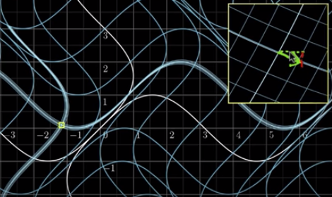
We have got this very non-linear transformation, and we see that if you zoom in on a specific point while that transformation is happening, it looks a lot like something linear and we can reason that you can figure out what linear transformation that looks like by taking the partial derivatives of your given function from above and then turning that into a matrix.
So if we calculate that we will get the following given $(-2, 1)$:
\[\begin{bmatrix} 1 & \cos(1) \\ \cos(-2) & 1 \end{bmatrix}\]Determinant
If we have a $2x2$ matrix, we can calculate the determinant as follows:
\[\begin{align} \det\begin{pmatrix}\begin{bmatrix}3 & 1\\0 & 2\end{bmatrix}\end{pmatrix} &= 3 * 2 - 1 * 0 \\\ &= 6 \end{align}\]Here we can see that the determinant records the stretched or squished space of the transformation.
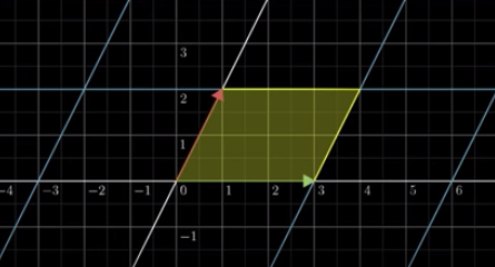
So, if we look at our starting point where we have a bases vectors and therefore a square shape of size $1x1$, we can see that is getting stretched by the factor of 6, the determinant we have calculated.
\[\begin{align} \det\begin{pmatrix}\begin{bmatrix}1 & \cos(1)\\\cos(-2) & 1\end{bmatrix}\end{pmatrix} &= 1 * 1 - 0.42 * 0.54 \\\ &= 1.227 \end{align}\]Python example
In python we can use either the sympy library or JAX.
from math import sin
from math import cos
from sympy import Matrix
from sympy.abc import rho
from sympy.abc import phi

X = Matrix([rho * cos(phi), rho * sin(phi), pow(rho, 2)])
Y = Matrix([rho, phi])

X.jacobian(Y)
import jax.numpy as np
from jax import grad
from jax import jvp

x = np.array([5, 3], dtype=float)

def cost(x):
    return pow(x[0], 2) / x[1] - np.log(x[1])

gradient_cost = grad(cost)
jacobian_cost = jvp(cost)

gradient_cost(x)
jacobian_cost(np.array([x, x, x]))
Conclusion
If we know the matrix that describes the transformation, the determinant of that matrix will tell us the factor by which the area will get stretched or squished. That is what this Jacobian determinant is.